Migrate GeoNode Base URL
The migrate_baseurl Management Command allows you to fix all the GeoNode Links whenever, for some reason,
you need to change the Domain Name of IP Address of GeoNode.
This must be used also in the cases you’ll need to change the network schema from HTTP to HTTPS, as an instance.
First of all let’s take a look at the –help option of the migrate_baseurl
management command in order to inspect all the command options and features.
Run
DJANGO_SETTINGS_MODULE=geonode.settings python manage.py migrate_baseurl --help
This will produce output that looks like the following
usage: manage.py migrate_baseurl [-h] [--version] [-v {0,1,2,3}]
                             [--settings SETTINGS]
                             [--pythonpath PYTHONPATH] [--traceback]
                             [--no-color] [-f]
                             [--source-address SOURCE_ADDRESS]
                             [--target-address TARGET_ADDRESS]

Migrate GeoNode VM Base URL

optional arguments:
-h, --help            show this help message and exit
--version             show program's version number and exit
-v {0,1,2,3}, --verbosity {0,1,2,3}
                        Verbosity level; 0=minimal output, 1=normal output,
                        2=verbose output, 3=very verbose output
--settings SETTINGS   The Python path to a settings module, e.g.
                        "myproject.settings.main". If this isn't provided, the
                        DJANGO_SETTINGS_MODULE environment variable will be
                        used.
--pythonpath PYTHONPATH
                        A directory to add to the Python path, e.g.
                        "/home/djangoprojects/myproject".
--traceback           Raise on CommandError exceptions
--no-color            Don't colorize the command output.
-f, --force           Forces the execution without asking for confirmation.
--source-address SOURCE_ADDRESS
                        Source Address (the one currently on DB e.g.
                        http://192.168.1.23)
--target-address TARGET_ADDRESS
                        Target Address (the one to be changed e.g. http://my-
                        public.geonode.org)
Example 1: I want to move my GeoNode instance from
http:\\127.0.0.1tohttp:\\example.orgWarning
Make always sure you are using the correct settings
DJANGO_SETTINGS_MODULE=geonode.settings python manage.py migrate_baseurl --source-address=127.0.0.1 --target-address=example.org
Example 2: I want to move my GeoNode instance from
http:\\example.orgtohttps:\\example.orgWarning
Make always sure you are using the correct settings
DJANGO_SETTINGS_MODULE=geonode.settings python manage.py migrate_baseurl --source-address=http:\\example.org --target-address=https:\\example.org
Example 3: I want to move my GeoNode instance from
https:\\example.orgtohttps:\\geonode.example.orgWarning
Make always sure you are using the correct settings
DJANGO_SETTINGS_MODULE=geonode.settings python manage.py migrate_baseurl --source-address=example.org --target-address=geonode.example.org
Note
After migrating the base URL, make sure to sanitize the links and catalog metadata also (Update Permissions, Metadata, Legends and Download Links).
Update Permissions, Metadata, Legends and Download Links
The following three utility Management Commands, allow to fixup:
Users/Groups Permissions on Datasets; those will be refreshed and synchronized with the GIS Server ones also
Metadata, Legend and Download links on Datasets and Maps
Cleanup Duplicated Links and Outdated Thumbnails
Management Command sync_geonode_datasets
This command allows to sync already existing permissions on Datasets. In order to change/set Datasets’ permissions refer to the section Batch Sync Permissions
The options are:
filter; Only update data the Dataset names that match the given filter.
username; Only update data owned by the specified username.
updatepermissions; Update the Dataset permissions; synchronize it back to the GeoSpatial Server. This option is also available from the Layer Details page.
updateattributes; Update the Dataset attributes; synchronize it back to the GeoSpatial Server. This option is also available from the Layer Details page.
updatethumbnails; Update the Dataset thumbnail. This option is also available from the Layer Details page.
updatebbox; Update the Dataset BBOX and LotLan BBOX. This option is also available from the Layer Details page.
remove-duplicates; Removes duplicated Links.
First of all let’s take a look at the –help option of the sync_geonode_datasets
management command in order to inspect all the command options and features.
Run
DJANGO_SETTINGS_MODULE=geonode.settings python manage.py sync_geonode_datasets --help
Note
If you enabled local_settings.py the command will change as following:
DJANGO_SETTINGS_MODULE=geonode.local_settings python manage.py sync_geonode_datasets --help
This will produce output that looks like the following
usage: manage.py sync_geonode_datasets [-h] [--version] [-v {0,1,2,3}]
                                    [--settings SETTINGS]
                                    [--pythonpath PYTHONPATH] [--traceback]
                                    [--no-color] [-i] [-d] [-f FILTER]
                                    [-u USERNAME] [--updatepermissions]
                                    [--updatethumbnails] [--updateattributes][--updatebbox]

Update the GeoNode Datasets: permissions (including GeoFence database),
statistics, thumbnails

optional arguments:
-h, --help            show this help message and exit
--version             show program's version number and exit
-v {0,1,2,3}, --verbosity {0,1,2,3}
                        Verbosity level; 0=minimal output, 1=normal output,
                        2=verbose output, 3=very verbose output
--settings SETTINGS   The Python path to a settings module, e.g.
                        "myproject.settings.main". If this isn't provided, the
                        DJANGO_SETTINGS_MODULE environment variable will be
                        used.
--pythonpath PYTHONPATH
                        A directory to add to the Python path, e.g.
                        "/home/djangoprojects/myproject".
--traceback           Raise on CommandError exceptions
--no-color            Don't colorize the command output.
-i, --ignore-errors   Stop after any errors are encountered.
-d, --remove-duplicates
                        Remove duplicates first.
-f FILTER, --filter FILTER
                        Only update data the Datasets that match the given
                        filter.
-u USERNAME, --username USERNAME
                        Only update data owned by the specified username.
--updatepermissions   Update the Dataset permissions.
--updatethumbnails    Update the Dataset styles and thumbnails.
--updateattributes    Update the Dataset attributes.
--updatebbox          Update the Dataset BBOX.
Example 1: I want to update/sync all Datasets permissions and attributes with the GeoSpatial Server
Warning
Make always sure you are using the correct settings
DJANGO_SETTINGS_MODULE=geonode.settings python manage.py sync_geonode_datasets --updatepermissions --updateattributes
Example 2: I want to regenerate the Thumbnails of all the Datasets belonging to
afabianiWarning
Make always sure you are using the correct settings
DJANGO_SETTINGS_MODULE=geonode.settings python manage.py sync_geonode_datasets -u afabiani --updatethumbnails
Management Command sync_geonode_maps
This command is basically similar to the previous one, but affects the Maps; with some limitations.
The options are:
filter; Only update data the maps titles that match the given filter.
username; Only update data owned by the specified username.
updatethumbnails; Update the map styles and thumbnails. This option is also available from the Map Details page.
remove-duplicates; Removes duplicated Links.
First of all let’s take a look at the –help option of the sync_geonode_maps
management command in order to inspect all the command options and features.
Run
DJANGO_SETTINGS_MODULE=geonode.settings python manage.py sync_geonode_maps --help
Note
If you enabled local_settings.py the command will change as following:
DJANGO_SETTINGS_MODULE=geonode.local_settings python manage.py sync_geonode_maps --help
This will produce output that looks like the following
usage: manage.py sync_geonode_maps [-h] [--version] [-v {0,1,2,3}]
                                [--settings SETTINGS]
                                [--pythonpath PYTHONPATH] [--traceback]
                                [--no-color] [-i] [-d] [-f FILTER]
                                [-u USERNAME] [--updatethumbnails]

Update the GeoNode maps: permissions, thumbnails

optional arguments:
-h, --help            show this help message and exit
--version             show program's version number and exit
-v {0,1,2,3}, --verbosity {0,1,2,3}
                        Verbosity level; 0=minimal output, 1=normal output,
                        2=verbose output, 3=very verbose output
--settings SETTINGS   The Python path to a settings module, e.g.
                        "myproject.settings.main". If this isn't provided, the
                        DJANGO_SETTINGS_MODULE environment variable will be
                        used.
--pythonpath PYTHONPATH
                        A directory to add to the Python path, e.g.
                        "/home/djangoprojects/myproject".
--traceback           Raise on CommandError exceptions
--no-color            Don't colorize the command output.
-i, --ignore-errors   Stop after any errors are encountered.
-d, --remove-duplicates
                        Remove duplicates first.
-f FILTER, --filter FILTER
                        Only update data the maps that match the given filter.
-u USERNAME, --username USERNAME
                        Only update data owned by the specified username.
--updatethumbnails    Update the map styles and thumbnails.
Example 1: I want to regenerate the Thumbnail of the Map
This is a test MapWarning
Make always sure you are using the correct settings
DJANGO_SETTINGS_MODULE=geonode.settings python manage.py sync_geonode_maps --updatethumbnails -f 'This is a test Map'
Management Command set_all_datasets_metadata
This command allows to reset Metadata Attributes and Catalogue Schema on Datasets. The command will also update the CSW Catalogue XML and Links of GeoNode.
The options are:
filter; Only update data the Datasets that match the given filter.
username; Only update data owned by the specified username.
remove-duplicates; Update the map styles and thumbnails.
delete-orphaned-thumbs; Removes duplicated Links.
set-uuid; will refresh the UUID based on the UUID_HANDLER if configured (Default False).
set_attrib; If set will refresh the attributes of the resource taken from Geoserver. (Default True).
set_links; If set will refresh the links of the resource. (Default True).
First of all let’s take a look at the –help option of the set_all_datasets_metadata
management command in order to inspect all the command options and features.
Run
DJANGO_SETTINGS_MODULE=geonode.settings python manage.py set_all_datasets_metadata --help
Note
If you enabled local_settings.py the command will change as following:
DJANGO_SETTINGS_MODULE=geonode.local_settings python manage.py set_all_datasets_metadata --help
This will produce output that looks like the following
usage: manage.py set_all_datasets_metadata [-h] [--version] [-v {0,1,2,3}]
                                        [--settings SETTINGS]
                                        [--pythonpath PYTHONPATH]
                                        [--traceback] [--no-color] [-i] [-d]
                                        [-t] [-f FILTER] [-u USERNAME]

Resets Metadata Attributes and Schema to All Datasets

optional arguments:
-h, --help            show this help message and exit
--version             show program's version number and exit
-v {0,1,2,3}, --verbosity {0,1,2,3}
                        Verbosity level; 0=minimal output, 1=normal output,
                        2=verbose output, 3=very verbose output
--settings SETTINGS   The Python path to a settings module, e.g.
                        "myproject.settings.main". If this isn't provided, the
                        DJANGO_SETTINGS_MODULE environment variable will be
                        used.
--pythonpath PYTHONPATH
                        A directory to add to the Python path, e.g.
                        "/home/djangoprojects/myproject".
--traceback           Raise on CommandError exceptions
--no-color            Don't colorize the command output.
-i, --ignore-errors   Stop after any errors are encountered.
-d, --remove-duplicates
                        Remove duplicates first.
-t, --delete-orphaned-thumbs
                        Delete Orphaned Thumbnails.
-f FILTER, --filter FILTER
                        Only update data the Datasets that match the given
                        filter
-u USERNAME, --username USERNAME
                        Only update data owned by the specified username
Example 1: After having changed the Base URL, I want to regenerate all the Catalogue Schema and eventually remove all duplicates.
Warning
Make always sure you are using the correct settings
DJANGO_SETTINGS_MODULE=geonode.settings python manage.py set_all_datasets_metadata -d
Loading Data into GeoNode
There are situations where it is not possible or not convenient to use the Upload Form to add new Datasets to GeoNode via the web interface. For instance:
The dataset is too big to be uploaded through a web interface.
Import data from a mass storage programmatically.
Import tables from a database.
This section will walk you through the various options available to load data into your GeoNode from GeoServer, from the command-line or programmatically.
Warning
Some parts of this section have been taken from the GeoServer project and training documentation.
Management Command importlayers
The geonode.geoserver Django app includes 2 management commands that you can use to
load data in your GeoNode.
Both of them can be invoked by using the manage.py script.
First of all let’s take a look at the –help option of the importlayers
management command in order to inspect all the command options and features.
Run
DJANGO_SETTINGS_MODULE=geonode.settings python manage.py importlayers --help
Note
If you enabled local_settings.py the command will change as following:
DJANGO_SETTINGS_MODULE=geonode.local_settings python manage.py importlayers --help
This will produce output that looks like the following
usage: manage.py importlayers [-h] [-hh HOST] [-u USERNAME] [-p PASSWORD]
                              [--version] [-v {0,1,2,3}] [--settings SETTINGS]
                              [--pythonpath PYTHONPATH] [--traceback] [--no-color]
                              [--force-color] [--skip-checks]
                              [path [path ...]]

Brings files from a local directory, including subfolders, into a GeoNode site.
The datasets are added to the Django database, the GeoServer configuration, and the
pycsw metadata index. At this moment only files of type Esri Shapefile (.shp) and GeoTiff (.tif) are supported.
In order to perform the import, GeoNode must be up and running.

positional arguments:
path                  path [path...]

optional arguments:
-h, --help            show this help message and exit
--version             show program's version number and exit
-v {0,1,2,3}, --verbosity {0,1,2,3}
                        Verbosity level; 0=minimal output, 1=normal output,
                        2=verbose output, 3=very verbose output
--settings SETTINGS   The Python path to a settings module, e.g.
                        "myproject.settings.main". If this isn't provided, the
                        DJANGO_SETTINGS_MODULE environment variable will be
                        used.
--pythonpath PYTHONPATH
                        A directory to add to the Python path, e.g.
                        "/home/djangoprojects/myproject".
-hh HOST, --host HOST
                        Geonode host url
-u USERNAME, --username USERNAME
                        Geonode username
-p PASSWORD, --password PASSWORD
                        Geonode password
While the description of most of the options should be self explanatory, its worth reviewing some of the key options a bit more in details.
The -hh Identifies the GeoNode server where we want to upload our Datasets. The default value is http://localhost:8000.
The -u Identifies the username for the login. The default value is admin.
The -p Identifies the password for the login. The default value is admin.
The import Datasets management command is invoked by specifying options as described above and specifying the path to a directory that contains multiple files. For purposes of this exercise, let’s use the default set of testing Datasets that ship with geonode. You can replace this path with a directory to your own shapefiles.
This command will produce the following output to your terminal
san_andres_y_providencia_poi.shp: 201
san_andres_y_providencia_location.shp: 201
san_andres_y_providencia_administrative.shp: 201
san_andres_y_providencia_coastline.shp: 201
san_andres_y_providencia_highway.shp: 201
single_point.shp: 201
san_andres_y_providencia_water.shp: 201
san_andres_y_providencia_natural.shp: 201

1.7456605294117646 seconds per Dataset

Output data: {
    "success": [
        "san_andres_y_providencia_poi.shp",
        "san_andres_y_providencia_location.shp",
        "san_andres_y_providencia_administrative.shp",
        "san_andres_y_providencia_coastline.shp",
        "san_andres_y_providencia_highway.shp",
        "single_point.shp",
        "san_andres_y_providencia_water.shp",
        "san_andres_y_providencia_natural.shp"
    ],
    "errors": []
}
As output the command will print:
The status code, is the response coming from GeoNode. For example 201 means that the Dataset has been correctly uploaded
If you encounter errors while running this command, please check the GeoNode logs for more information.
Management Command updatelayers
While it is possible to import Datasets directly from your servers filesystem into your GeoNode, you may have an existing GeoServer that already has data in it, or you may want to configure data from a GeoServer which is not directly supported by uploading data.
GeoServer supports a wide range of data formats and connections to database, some of them may not be supported as GeoNode upload formats. You can add them to your GeoNode by following the procedure described below.
GeoServer supports 4 types of data: Raster, Vector, Databases and Cascaded.
For a list of the supported formats for each type of data, consult the following pages:
https://docs.geoserver.org/latest/en/user/data/vector/index.html
https://docs.geoserver.org/latest/en/user/data/raster/index.html
https://docs.geoserver.org/latest/en/user/data/database/index.html
https://docs.geoserver.org/latest/en/user/data/cascaded/index.html
Note
Some of these raster or vector formats or database types require that you install specific plugins in your GeoServer in order to use the. Please consult the GeoServer documentation for more information.
Data from a PostGIS database
Lets walk through an example of configuring a new PostGIS database in GeoServer and then configuring those Datasets in your GeoNode.
First visit the GeoServer administration interface on your server. This is usually on port 8080 and is available at http://localhost:8080/geoserver/web/
You should login with the superuser credentials you setup when you first configured your GeoNode instance.
Once you are logged in to the GeoServer Admin interface, you should see the following.
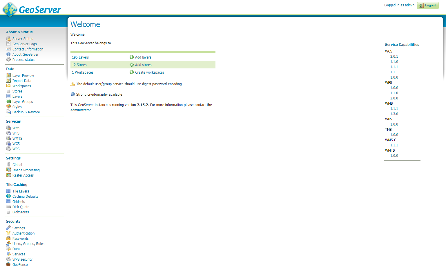
Note
The number of stores, Datasets and workspaces may be different depending on what you already have configured in your GeoServer.
Next you want to select the “Stores” option in the left hand menu, and then the “Add new Store” option. The following screen will be displayed.
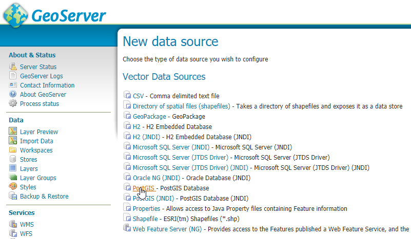
In this case, we want to select the PostGIS store type to create a connection to our existing database. On the next screen you will need to enter the parameters to connect to your PostGIS database (alter as necessary for your own database).
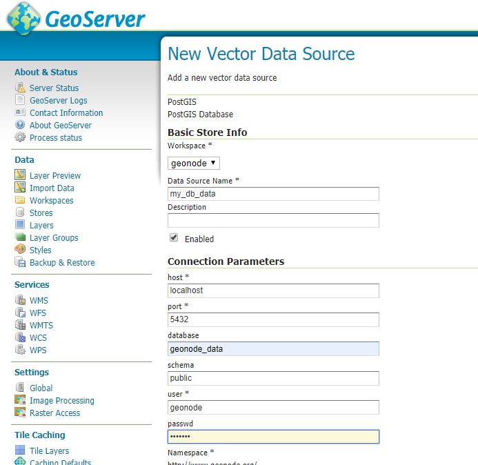
Note
If you are unsure about any of the settings, leave them as the default.
The next screen lets you configure the Datasets in your database. This will of course be different depending on the Datasets in your database.

Select the “Publish” button for one of the Datasets and the next screen will be displayed where you can enter metadata for this Dataset. Since we will be managing this metadata in GeoNode, we can leave these alone for now.
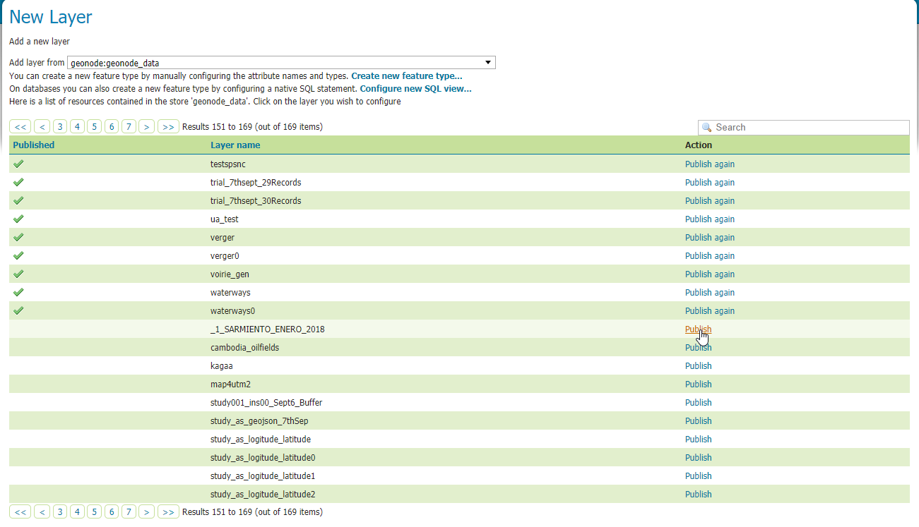
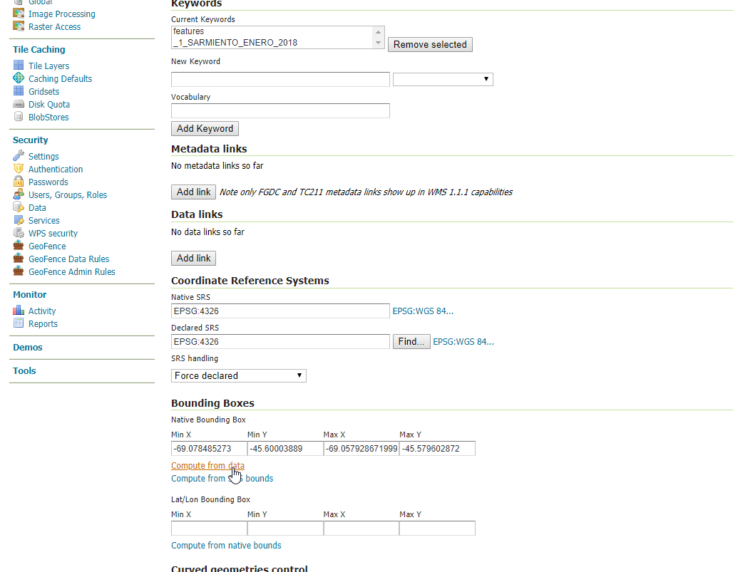
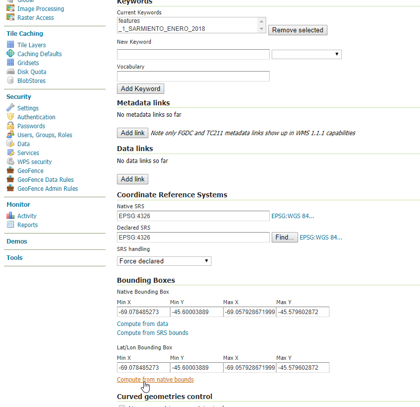
The things that must be specified are the Declared SRS and you must select the “Compute from Data” and “Compute from native bounds” links after the SRS is specified.
Click save and this Dataset will now be configured for use in your GeoServer.
The next step is to configure these Datasets in GeoNode. The
updatelayersmanagement command can be used for this purpose. As withimportlayers, it’s useful to look at the command line options for this command by passing the –help optionRun
DJANGO_SETTINGS_MODULE=geonode.settings python manage.py updatelayers --help
Note
If you enabled
local_settings.pythe command will change as following:DJANGO_SETTINGS_MODULE=geonode.local_settings python manage.py updatelayers --help
This will produce output that looks like the following
usage: manage.py updatelayers [-h] [--version] [-v {0,1,2,3}]
                            [--settings SETTINGS] [--pythonpath PYTHONPATH]
                            [--traceback] [--no-color] [-i]
                            [--skip-unadvertised]
                            [--skip-geonode-registered] [--remove-deleted]
                            [-u USER] [-f FILTER] [-s STORE] [-w WORKSPACE]
                            [-p PERMISSIONS]

Update the GeoNode application with data from GeoServer

optional arguments:
-h, --help            show this help message and exit
--version             show program's version number and exit
-v {0,1,2,3}, --verbosity {0,1,2,3}
                        Verbosity level; 0=minimal output, 1=normal output,
                        2=verbose output, 3=very verbose output
--settings SETTINGS   The Python path to a settings module, e.g.
                        "myproject.settings.main". If this isn't provided, the
                        DJANGO_SETTINGS_MODULE environment variable will be
                        used.
--pythonpath PYTHONPATH
                        A directory to add to the Python path, e.g.
                        "/home/djangoprojects/myproject".
--traceback           Raise on CommandError exceptions
--no-color            Don't colorize the command output.
-i, --ignore-errors   Stop after any errors are encountered.
--skip-unadvertised   Skip processing unadvertised Datasets from GeoSever.
--skip-geonode-registered
                        Just processing GeoServer Datasets still not registered
                        in GeoNode.
--remove-deleted      Remove GeoNode Datasets that have been deleted from
                        GeoSever.
-u USER, --user USER  Name of the user account which should own the imported
                        Datasets
-f FILTER, --filter FILTER
                        Only update data the Datasets that match the given
                        filter
-s STORE, --store STORE
                        Only update data the Datasets for the given geoserver
                        store name
-w WORKSPACE, --workspace WORKSPACE
                        Only update data on specified workspace
-p PERMISSIONS, --permissions PERMISSIONS
                        Permissions to apply to each Dataset
The update procedure includes the following steps:
The process fetches from GeoServer the relevant WMS layers (all, by store or by workspace)
If a filter is defined, the GeoServer layers are filtered
For each of the layers, a GeoNode dataset is created based on the metadata registered on GeoServer (title, abstract, bounds)
New layers are added, existing layers are replaced, unless the –skip-geonode-registered option is used
The GeoNode layers, added in previous runs of the update process, which are no longer available in GeoServer are removed, if the –remove-delete option is set
Warning
One of the –workspace or –store must be always specified if you want to ingest Datasets belonging to a specific Workspace. As an instance, in order to ingest the Datasets present into the geonode workspace, you will need to specify the option -w geonode.
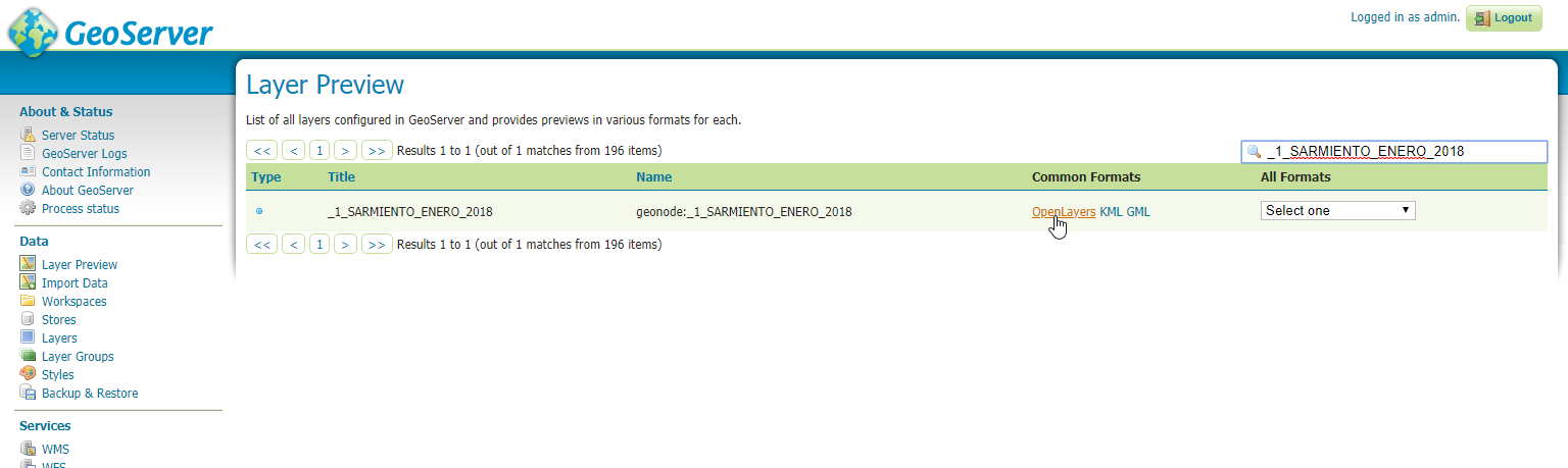
Let’s ingest the Dataset
geonode:_1_SARMIENTO_ENERO_2018from thegeonodeworkspace.DJANGO_SETTINGS_MODULE=geonode.settings python manage.py updatelayers -w geonode -f _1_SARMIENTO_ENERO_2018
Inspecting the available Datasets in GeoServer ...
Found 1 Datasets, starting processing
/usr/local/lib/python2.7/site-packages/owslib/iso.py:117: FutureWarning: the .identification and .serviceidentification properties will merge into .identification being a list of properties.  This is currently implemented in .identificationinfo.  Please see https://github.com/geopython/OWSLib/issues/38 for more information
FutureWarning)
/usr/local/lib/python2.7/site-packages/owslib/iso.py:495: FutureWarning: The .keywords and .keywords2 properties will merge into the .keywords property in the future, with .keywords becoming a list of MD_Keywords instances. This is currently implemented in .keywords2. Please see https://github.com/geopython/OWSLib/issues/301 for more information
FutureWarning)
Content-Type: text/html; charset="utf-8"
MIME-Version: 1.0
Content-Transfer-Encoding: 7bit
Subject: [master.demo.geonode.org] A new Dataset has been uploaded
From: webmaster@localhost
To: mapadeldelito@chubut.gov.ar
Reply-To: webmaster@localhost
Date: Tue, 08 Oct 2019 12:26:17 -0000
Message-ID: <20191008122617.28801.94967@d3cf85425231>


<body>
You have received the following notice from master.demo.geonode.org:
<p>

The user <i><a href="http://master.demo.geonode.org/people/profile/admin">admin</a></i> uploaded the following Dataset:<br/>
<strong>_1_SARMIENTO_ENERO_2018</strong><br/>
You can visit the Dataset's detail page here: http://master.demo.geonode.org/Datasets/geonode:_1_SARMIENTO_ENERO_2018

</p>
<p>
To change how you receive notifications, please go to http://master.demo.geonode.org
</p>
</body>

-------------------------------------------------------------------------------
Content-Type: text/html; charset="utf-8"
MIME-Version: 1.0
Content-Transfer-Encoding: 7bit
Subject: [master.demo.geonode.org] A new Dataset has been uploaded
From: webmaster@localhost
To: giacomo8vinci@gmail.com
Reply-To: webmaster@localhost
Date: Tue, 08 Oct 2019 12:26:17 -0000
Message-ID: <20191008122617.28801.53784@d3cf85425231>


<body>
You have received the following notice from master.demo.geonode.org:
<p>

The user <i><a href="http://master.demo.geonode.org/people/profile/admin">admin</a></i> uploaded the following Dataset:<br/>
<strong>_1_SARMIENTO_ENERO_2018</strong><br/>
You can visit the Dataset's detail page here: http://master.demo.geonode.org/Datasets/geonode:_1_SARMIENTO_ENERO_2018

</p>
<p>
To change how you receive notifications, please go to http://master.demo.geonode.org
</p>
</body>

-------------------------------------------------------------------------------
Content-Type: text/html; charset="utf-8"
MIME-Version: 1.0
Content-Transfer-Encoding: 7bit
Subject: [master.demo.geonode.org] A new Dataset has been uploaded
From: webmaster@localhost
To: fmgagliano@gmail.com
Reply-To: webmaster@localhost
Date: Tue, 08 Oct 2019 12:26:17 -0000
Message-ID: <20191008122617.28801.26265@d3cf85425231>


<body>
You have received the following notice from master.demo.geonode.org:
<p>

The user <i><a href="http://master.demo.geonode.org/people/profile/admin">admin</a></i> uploaded the following Dataset:<br/>
<strong>_1_SARMIENTO_ENERO_2018</strong><br/>
You can visit the Dataset's detail page here: http://master.demo.geonode.org/Datasets/geonode:_1_SARMIENTO_ENERO_2018

</p>
<p>
To change how you receive notifications, please go to http://master.demo.geonode.org
</p>
</body>

-------------------------------------------------------------------------------
Found geoserver resource for this Dataset: _1_SARMIENTO_ENERO_2018
... Creating Default Resource Links for Layer [geonode:_1_SARMIENTO_ENERO_2018]
-- Resource Links[Prune old links]...
-- Resource Links[Prune old links]...done!
-- Resource Links[Compute parameters for the new links]...
-- Resource Links[Create Raw Data download link]...
-- Resource Links[Create Raw Data download link]...done!
-- Resource Links[Set download links for WMS, WCS or WFS and KML]...
-- Resource Links[Set download links for WMS, WCS or WFS and KML]...done!
-- Resource Links[Legend link]...
-- Resource Links[Legend link]...done!
-- Resource Links[Thumbnail link]...
-- Resource Links[Thumbnail link]...done!
-- Resource Links[OWS Links]...
-- Resource Links[OWS Links]...done!
Content-Type: text/html; charset="utf-8"
MIME-Version: 1.0
Content-Transfer-Encoding: 7bit
Subject: [master.demo.geonode.org] A Dataset has been updated
From: webmaster@localhost
To: mapadeldelito@chubut.gov.ar
Reply-To: webmaster@localhost
Date: Tue, 08 Oct 2019 12:26:20 -0000
Message-ID: <20191008122620.28801.81598@d3cf85425231>


<body>
You have received the following notice from master.demo.geonode.org:
<p>

The following Dataset was updated:<br/>
<strong>_1_SARMIENTO_ENERO_2018</strong>, owned by <i><a href="http://master.demo.geonode.org/people/profile/admin">admin</a></i><br/>
You can visit the Dataset's detail page here: http://master.demo.geonode.org/Datasets/geonode:_1_SARMIENTO_ENERO_2018

</p>
<p>
To change how you receive notifications, please go to http://master.demo.geonode.org
</p>
</body>

-------------------------------------------------------------------------------
Content-Type: text/html; charset="utf-8"
MIME-Version: 1.0
Content-Transfer-Encoding: 7bit
Subject: [master.demo.geonode.org] A Dataset has been updated
From: webmaster@localhost
To: giacomo8vinci@gmail.com
Reply-To: webmaster@localhost
Date: Tue, 08 Oct 2019 12:26:20 -0000
Message-ID: <20191008122620.28801.93778@d3cf85425231>


<body>
You have received the following notice from master.demo.geonode.org:
<p>

The following Dataset was updated:<br/>
<strong>_1_SARMIENTO_ENERO_2018</strong>, owned by <i><a href="http://master.demo.geonode.org/people/profile/admin">admin</a></i><br/>
You can visit the Dataset's detail page here: http://master.demo.geonode.org/Datasets/geonode:_1_SARMIENTO_ENERO_2018

</p>
<p>
To change how you receive notifications, please go to http://master.demo.geonode.org
</p>
</body>

-------------------------------------------------------------------------------
Content-Type: text/html; charset="utf-8"
MIME-Version: 1.0
Content-Transfer-Encoding: 7bit
Subject: [master.demo.geonode.org] A Dataset has been updated
From: webmaster@localhost
To: fmgagliano@gmail.com
Reply-To: webmaster@localhost
Date: Tue, 08 Oct 2019 12:26:20 -0000
Message-ID: <20191008122620.28801.58585@d3cf85425231>


<body>
You have received the following notice from master.demo.geonode.org:
<p>

The following Dataset was updated:<br/>
<strong>_1_SARMIENTO_ENERO_2018</strong>, owned by <i><a href="http://master.demo.geonode.org/people/profile/admin">admin</a></i><br/>
You can visit the Dataset's detail page here: http://master.demo.geonode.org/Datasets/geonode:_1_SARMIENTO_ENERO_2018

</p>
<p>
To change how you receive notifications, please go to http://master.demo.geonode.org
</p>
</body>

-------------------------------------------------------------------------------
Found geoserver resource for this Dataset: _1_SARMIENTO_ENERO_2018
/usr/local/lib/python2.7/site-packages/geoserver/style.py:80: FutureWarning: The behavior of this method will change in future versions.  Use specific 'len(elem)' or 'elem is not None' test instead.
if not user_style:
/usr/local/lib/python2.7/site-packages/geoserver/style.py:84: FutureWarning: The behavior of this method will change in future versions.  Use specific 'len(elem)' or 'elem is not None' test instead.
if user_style:
... Creating Default Resource Links for Layer [geonode:_1_SARMIENTO_ENERO_2018]
-- Resource Links[Prune old links]...
-- Resource Links[Prune old links]...done!
-- Resource Links[Compute parameters for the new links]...
-- Resource Links[Create Raw Data download link]...
-- Resource Links[Create Raw Data download link]...done!
-- Resource Links[Set download links for WMS, WCS or WFS and KML]...
-- Resource Links[Set download links for WMS, WCS or WFS and KML]...done!
-- Resource Links[Legend link]...
-- Resource Links[Legend link]...done!
-- Resource Links[Thumbnail link]...
-- Resource Links[Thumbnail link]...done!
-- Resource Links[OWS Links]...
-- Resource Links[OWS Links]...done!
[created] Layer _1_SARMIENTO_ENERO_2018 (1/1)


Finished processing 1 Datasets in 5.0 seconds.

1 Created Datasets
0 Updated Datasets
0 Failed Datasets
5.000000 seconds per Dataset
Note
In case you don’t specify the -f option, the Datasets that already exists in your GeoNode will be just updated and the configuration synchronized between GeoServer and GeoNode.
Warning
When updating from GeoServer, the configuration on GeoNode will be changed!
Using GDAL and OGR to convert your Data for use in GeoNode
GeoNode supports uploading data in ESRI shapefiles, GeoTIFF, CSV, GeoJSON, ASCII-GRID and KML / KMZ formats (for the last three formats only if you are using the geonode.importer backend).
If your data is in other formats, you will need to convert it into one of these formats for use in GeoNode.
If your Raster data is not correctly processed, it might be almost unusable with GeoServer and GeoNode. You will need to process it using GDAL.
You need to make sure that you have the GDAL library installed on your system. On Ubuntu you can install this package with the following command:
sudo apt-get install gdal-bin
OGR (Vector Data)
OGR is used to manipulate vector data. In this example, we will use MapInfo .tab files and convert them to shapefiles with the ogr2ogr command. We will use sample MapInfo files from the website linked below.
http://services.land.vic.gov.au/landchannel/content/help?name=sampledata
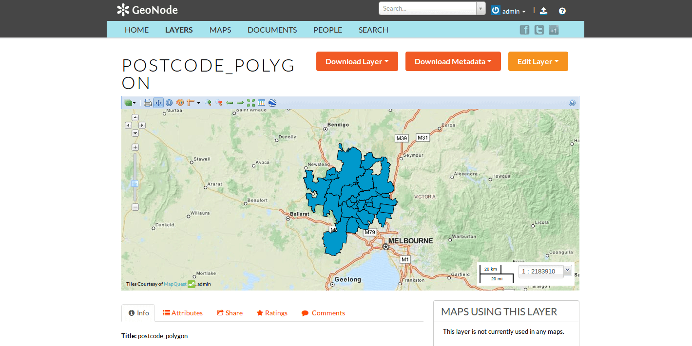
You can download the Admin;(Postcode) Dataset by issuing the following command:
$ wget http://services.land.vic.gov.au/sampledata/shape/admin_postcode_vm.zip
You will need to unzip this dataset by issuing the following command:
$ unzip admin_postcode_vm.zip
This will leave you with the following files in the directory where you executed the above commands:
|-- ANZVI0803003025.htm
|-- DSE_Data_Access_Licence.pdf
|-- VMADMIN.POSTCODE_POLYGON.xml
|-- admin_postcode_vm.zip
--- vicgrid94
    --- mif
        --- lga_polygon
            --- macedon\ ranges
                |-- EXTRACT_POLYGON.mid
                |-- EXTRACT_POLYGON.mif
                --- VMADMIN
                    |-- POSTCODE_POLYGON.mid
                    --- POSTCODE_POLYGON.mif
First, lets inspect this file set using the following command:
$ ogrinfo -so vicgrid94/mif/lga_polygon/macedon\ ranges/VMADMIN/POSTCODE_POLYGON.mid POSTCODE_POLYGON
The output will look like the following:
Had to open data source read-only.
INFO: Open of `vicgrid94/mif/lga_polygon/macedon ranges/VMADMIN/POSTCODE_POLYGON.mid'
    using driver `MapInfo File' successful.

Layer name: POSTCODE_POLYGON
Geometry: 3D Unknown (any)
Feature Count: 26
Extent: (2413931.249367, 2400162.366186) - (2508952.174431, 2512183.046927)
Layer SRS WKT:
PROJCS["unnamed",
    GEOGCS["unnamed",
        DATUM["GDA94",
            SPHEROID["GRS 80",6378137,298.257222101],
            TOWGS84[0,0,0,-0,-0,-0,0]],
        PRIMEM["Greenwich",0],
        UNIT["degree",0.0174532925199433]],
    PROJECTION["Lambert_Conformal_Conic_2SP"],
    PARAMETER["standard_parallel_1",-36],
    PARAMETER["standard_parallel_2",-38],
    PARAMETER["latitude_of_origin",-37],
    PARAMETER["central_meridian",145],
    PARAMETER["false_easting",2500000],
    PARAMETER["false_northing",2500000],
    UNIT["Meter",1]]
PFI: String (10.0)
POSTCODE: String (4.0)
FEATURE_TYPE: String (6.0)
FEATURE_QUALITY_ID: String (20.0)
PFI_CREATED: Date (10.0)
UFI: Real (12.0)
UFI_CREATED: Date (10.0)
UFI_OLD: Real (12.0)
This gives you information about the number of features, the extent, the projection and the attributes of this Dataset.
Next, lets go ahead and convert this Dataset into a shapefile by issuing the following command:
$ ogr2ogr -t_srs EPSG:4326 postcode_polygon.shp vicgrid94/mif/lga_polygon/macedon\ ranges/VMADMIN/POSTCODE_POLYGON.mid POSTCODE_POLYGON
Note that we have also reprojected the Dataset to the WGS84 spatial reference system with the -t_srs ogr2ogr option.
The output of this command will look like the following:
Warning 6: Normalized/laundered field name: 'FEATURE_TYPE' to 'FEATURE_TY'
Warning 6: Normalized/laundered field name: 'FEATURE_QUALITY_ID' to 'FEATURE_QU'
Warning 6: Normalized/laundered field name: 'PFI_CREATED' to 'PFI_CREATE'
Warning 6: Normalized/laundered field name: 'UFI_CREATED' to 'UFI_CREATE'
This output indicates that some of the field names were truncated to fit into the constraint that attributes in shapefiles are only 10 characters long.
You will now have a set of files that make up the postcode_polygon.shp shapefile set. We can inspect them by issuing the following command:
$ ogrinfo -so postcode_polygon.shp postcode_polygon
The output will look similar to the output we saw above when we inspected the MapInfo file we converted from:
INFO: Open of `postcode_polygon.shp'
      using driver `ESRI Shapefile' successful.

Layer name: postcode_polygon
Geometry: Polygon
Feature Count: 26
Extent: (144.030296, -37.898156) - (145.101137, -36.888878)
Layer SRS WKT:
GEOGCS["GCS_WGS_1984",
    DATUM["WGS_1984",
        SPHEROID["WGS_84",6378137,298.257223563]],
    PRIMEM["Greenwich",0],
    UNIT["Degree",0.017453292519943295]]
PFI: String (10.0)
POSTCODE: String (4.0)
FEATURE_TY: String (6.0)
FEATURE_QU: String (20.0)
PFI_CREATE: Date (10.0)
UFI: Real (12.0)
UFI_CREATE: Date (10.0)
UFI_OLD: Real (12.0)
These files can now be loaded into your GeoNode instance via the normal uploader.
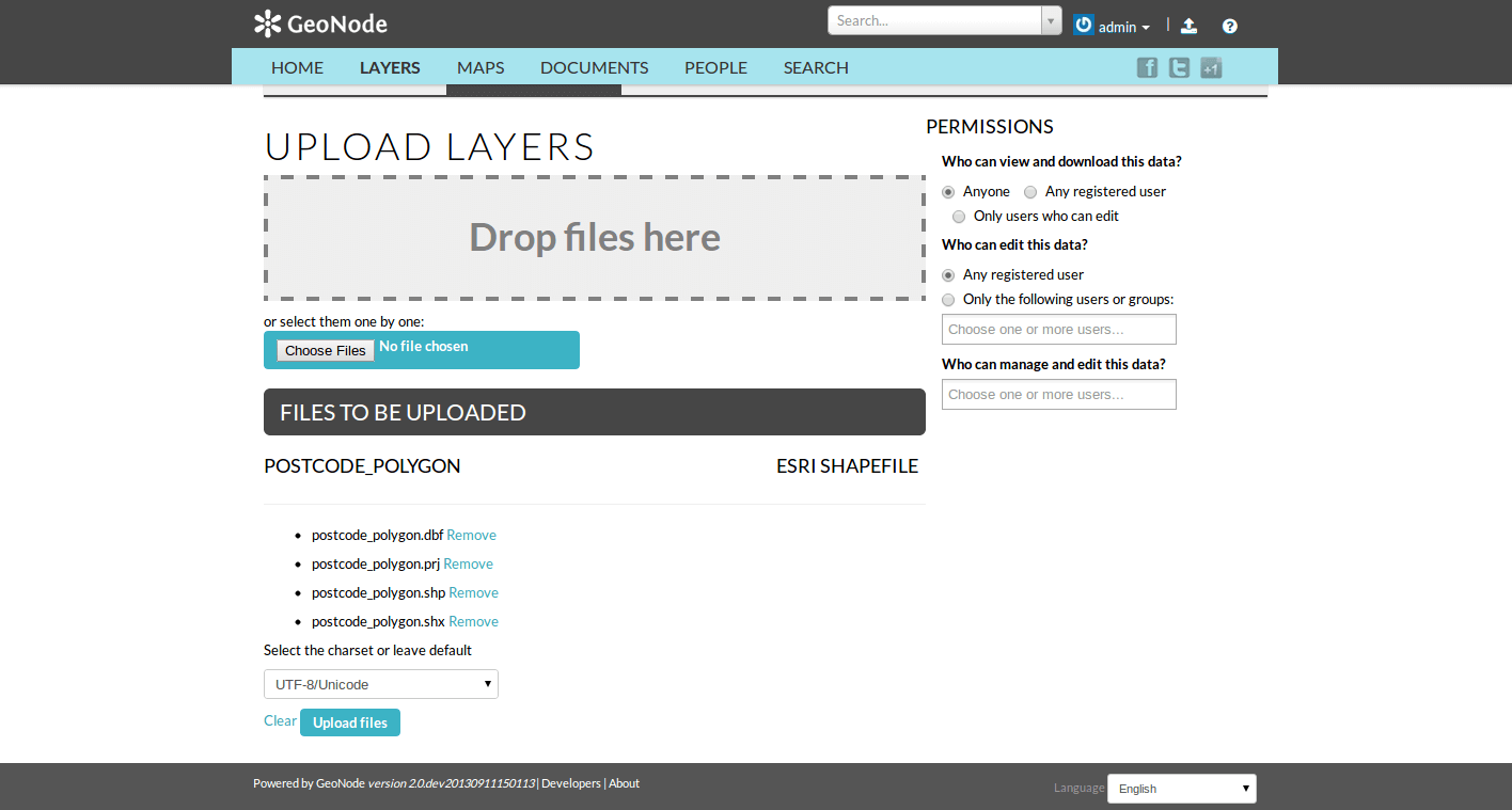
Visit the upload page in your GeoNode, drag and drop the files that composes the shapefile that you have generated using the GDAL ogr2ogr command (postcode_polygon.dbf, postcode_polygon.prj, postcode_polygon.shp, postcode_polygon.shx). Give the permissions as needed and then click the “Upload files” button.
As soon as the import process completes, you will have the possibility to go straight to the Dataset info page (“Layer Info” button), or to edit the metadata for that Dataset (“Edit Metadata” button), or to manage the styles for that Dataset (“Manage Styles”).
GDAL (Raster Data)
Let’s see several examples on how to either convert raster data into different formats and/or process it to get the best performances.
References:
https://geoserver.geo-solutions.it/edu/en/raster_data/processing.html
https://geoserver.geo-solutions.it/edu/en/raster_data/advanced_gdal/
Raster Data Conversion: Arc/Info Binary and ASCII Grid data into GeoTIFF format.
Let’s assume we have a sample ASCII Grid file compressed as an archive.
# Un-tar the files
tar -xvf sample_asc.tar
You will be left with the following files on your filesystem:
|-- batemans_ele
|   |-- dblbnd.adf
|   |-- hdr.adf
|   |-- metadata.xml
|   |-- prj.adf
|   |-- sta.adf
|   |-- w001001.adf
|   |-- w001001x.adf
|-- batemans_elevation.asc
The file batemans_elevation.asc is an Arc/Info ASCII Grid file and the files in
the batemans_ele directory are an Arc/Info Binary Grid file.
You can use the gdalinfo command to inspect both of these files by executing the
following command:
gdalinfo batemans_elevation.asc
The output should look like the following:
Driver: AAIGrid/Arc/Info ASCII Grid
Files: batemans_elevation.asc
Size is 155, 142
Coordinate System is `'
Origin = (239681.000000000000000,6050551.000000000000000)
Pixel Size = (100.000000000000000,-100.000000000000000)
Corner Coordinates:
Upper Left  (  239681.000, 6050551.000)
Lower Left  (  239681.000, 6036351.000)
Upper Right (  255181.000, 6050551.000)
Lower Right (  255181.000, 6036351.000)
Center      (  247431.000, 6043451.000)
Band 1 Block=155x1 Type=Float32, ColorInterp=Undefined
    NoData Value=-9999
You can then inspect the batemans_ele files by executing the following command:
gdalinfo batemans_ele
And this should be the corresponding output:
Driver: AIG/Arc/Info Binary Grid
Files: batemans_ele
    batemans_ele/dblbnd.adf
    batemans_ele/hdr.adf
    batemans_ele/metadata.xml
    batemans_ele/prj.adf
    batemans_ele/sta.adf
    batemans_ele/w001001.adf
    batemans_ele/w001001x.adf
Size is 155, 142
Coordinate System is:
PROJCS["unnamed",
    GEOGCS["GDA94",
        DATUM["Geocentric_Datum_of_Australia_1994",
            SPHEROID["GRS 1980",6378137,298.257222101,
                AUTHORITY["EPSG","7019"]],
            TOWGS84[0,0,0,0,0,0,0],
            AUTHORITY["EPSG","6283"]],
        PRIMEM["Greenwich",0,
            AUTHORITY["EPSG","8901"]],
        UNIT["degree",0.0174532925199433,
            AUTHORITY["EPSG","9122"]],
        AUTHORITY["EPSG","4283"]],
    PROJECTION["Transverse_Mercator"],
    PARAMETER["latitude_of_origin",0],
    PARAMETER["central_meridian",153],
    PARAMETER["scale_factor",0.9996],
    PARAMETER["false_easting",500000],
    PARAMETER["false_northing",10000000],
    UNIT["METERS",1]]
Origin = (239681.000000000000000,6050551.000000000000000)
Pixel Size = (100.000000000000000,-100.000000000000000)
Corner Coordinates:
Upper Left  (  239681.000, 6050551.000) (150d 7'28.35"E, 35d39'16.56"S)
Lower Left  (  239681.000, 6036351.000) (150d 7'11.78"E, 35d46'56.89"S)
Upper Right (  255181.000, 6050551.000) (150d17'44.07"E, 35d39'30.83"S)
Lower Right (  255181.000, 6036351.000) (150d17'28.49"E, 35d47'11.23"S)
Center      (  247431.000, 6043451.000) (150d12'28.17"E, 35d43'13.99"S)
Band 1 Block=256x4 Type=Float32, ColorInterp=Undefined
    Min=-62.102 Max=142.917
NoData Value=-3.4028234663852886e+38
You will notice that the batemans_elevation.asc file does not contain projection information while the batemans_ele file does.
Because of this, let’s use the batemans_ele files for this exercise and convert them to a GeoTiff for use in GeoNode.
We will also reproject this file into WGS84 in the process. This can be accomplished with the following command.
gdalwarp -t_srs EPSG:4326 batemans_ele batemans_ele.tif
The output will show you the progress of the conversion and when it is complete,
you will be left with a batemans_ele.tif file that you can upload to your GeoNode.
You can inspect this file with the gdalinfo command:
gdalinfo batemans_ele.tif
Which will produce the following output:
Driver: GTiff/GeoTIFF
Files: batemans_ele.tif
Size is 174, 130
Coordinate System is:
GEOGCS["WGS 84",
    DATUM["WGS_1984",
        SPHEROID["WGS 84",6378137,298.257223563,
            AUTHORITY["EPSG","7030"]],
        AUTHORITY["EPSG","6326"]],
    PRIMEM["Greenwich",0],
    UNIT["degree",0.0174532925199433],
    AUTHORITY["EPSG","4326"]]
Origin = (150.119938943722502,-35.654598806259330)
Pixel Size = (0.001011114155919,-0.001011114155919)
Metadata:
    AREA_OR_POINT=Area
Image Structure Metadata:
    INTERLEAVE=BAND
Corner Coordinates:
Upper Left  ( 150.1199389, -35.6545988) (150d 7'11.78"E, 35d39'16.56"S)
Lower Left  ( 150.1199389, -35.7860436) (150d 7'11.78"E, 35d47' 9.76"S)
Upper Right ( 150.2958728, -35.6545988) (150d17'45.14"E, 35d39'16.56"S)
Lower Right ( 150.2958728, -35.7860436) (150d17'45.14"E, 35d47' 9.76"S)
Center      ( 150.2079059, -35.7203212) (150d12'28.46"E, 35d43'13.16"S)
Band 1 Block=174x11 Type=Float32, ColorInterp=Gray
Raster Data Optimization: Optimizing and serving big raster data
(ref: https://geoserver.geo-solutions.it/edu/en/raster_data/advanced_gdal/example5.html)
When dealing with big raster datasets it could be very useful to use tiles.
Tiling allows large raster datasets to be broken-up into manageable pieces and are fundamental in defining and implementing a higher level raster I/O interface.
In this example we will use the original dataset of the chiangMai_ortho_optimized public raster Dataset which
is currently available on the Thai CHIANG MAI Urban Flooding GeoNode platform.
This dataset contains an orthorectified image stored as RGBa GeoTiff with 4 bands, three bands for the RGB and one for transparency (the alpha channel).
Calling the gdalinfo command to see detailed information:
gdalinfo chiangMai_ortho.tif
It will produce the following results:
Driver: GTiff/GeoTIFF
Files: chiangMai_ortho.tif
Size is 63203, 66211
Coordinate System is:
PROJCS["WGS 84 / UTM zone 47N",
    GEOGCS["WGS 84",
        DATUM["WGS_1984",
            SPHEROID["WGS 84",6378137,298.257223563,
                AUTHORITY["EPSG","7030"]],
            AUTHORITY["EPSG","6326"]],
        PRIMEM["Greenwich",0,
            AUTHORITY["EPSG","8901"]],
        UNIT["degree",0.0174532925199433,
            AUTHORITY["EPSG","9122"]],
        AUTHORITY["EPSG","4326"]],
    PROJECTION["Transverse_Mercator"],
    PARAMETER["latitude_of_origin",0],
    PARAMETER["central_meridian",99],
    PARAMETER["scale_factor",0.9996],
    PARAMETER["false_easting",500000],
    PARAMETER["false_northing",0],
    UNIT["metre",1,
        AUTHORITY["EPSG","9001"]],
    AXIS["Easting",EAST],
    AXIS["Northing",NORTH],
    AUTHORITY["EPSG","32647"]]
Origin = (487068.774750000040513,2057413.889810000080615)
Pixel Size = (0.028850000000000,-0.028850000000000)
Metadata:
AREA_OR_POINT=Area
TIFFTAG_SOFTWARE=pix4dmapper
Image Structure Metadata:
COMPRESSION=LZW
INTERLEAVE=PIXEL
Corner Coordinates:
Upper Left  (  487068.775, 2057413.890) ( 98d52'38.72"E, 18d36'27.34"N)
Lower Left  (  487068.775, 2055503.702) ( 98d52'38.77"E, 18d35'25.19"N)
Upper Right (  488892.181, 2057413.890) ( 98d53'40.94"E, 18d36'27.38"N)
Lower Right (  488892.181, 2055503.702) ( 98d53'40.98"E, 18d35'25.22"N)
Center      (  487980.478, 2056458.796) ( 98d53' 9.85"E, 18d35'56.28"N)
Band 1 Block=63203x1 Type=Byte, ColorInterp=Red
NoData Value=-10000
Mask Flags: PER_DATASET ALPHA
Band 2 Block=63203x1 Type=Byte, ColorInterp=Green
NoData Value=-10000
Mask Flags: PER_DATASET ALPHA
Band 3 Block=63203x1 Type=Byte, ColorInterp=Blue
NoData Value=-10000
Mask Flags: PER_DATASET ALPHA
Band 4 Block=63203x1 Type=Byte, ColorInterp=Alpha
NoData Value=-10000
As you can see, this GeoTiff has not been tiled. For accessing subsets though, tiling can make a difference. With tiling, data are stored and compressed in blocks (tiled) rather than line by line (stripped).
In the command output above it is visible that each band has blocks with the same width of the image (63203) and a unit length. The grids in the picture below show an image with equally sized tiles (left) and the same number of strips (right). To read data from the red subset, the intersected area will have to be decompressed.
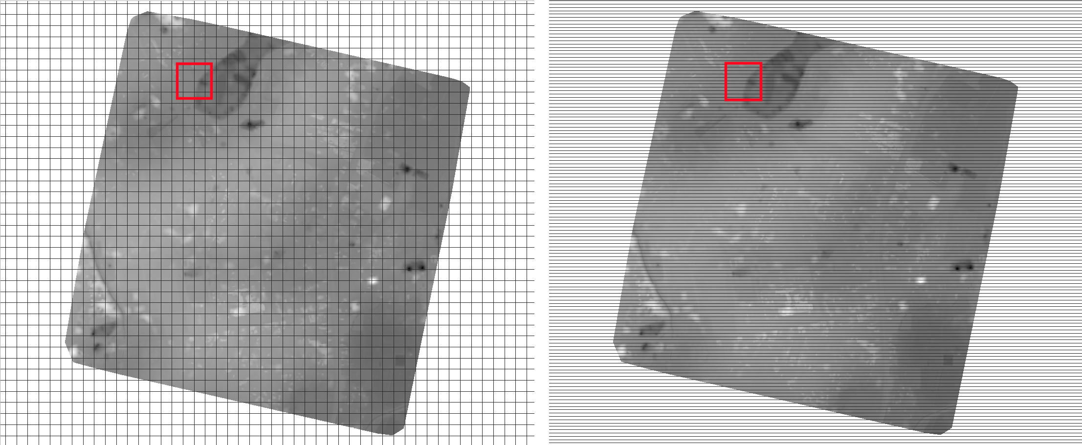
In the tiled image we will have to decompress only 16 tiles, whereas in the stripped image on the right we’ll have to decompress many more strips.
Drone images data usually have a stripped structure so, in most cases, they need to be optimized to increase performances.
Let’s take a look at the gdal_translate command used to optimize our GeoTiff:
gdal_translate -co TILED=YES -co COMPRESS=JPEG -co PHOTOMETRIC=YCBCR
            --config GDAL_TIFF_INTERNAL_MASK YES -b 1 -b 2 -b 3 -mask 4
            chiangMai_ortho.tif
            chiangMai_ortho_optimized.tif
Note
For the details about the command parameters see https://geoserver.geo-solutions.it/edu/en/raster_data/advanced_gdal/example5.html
Once the process ended, call the gdalinfo command on the resulting tif file:
gdalinfo chiangMai_ortho_optimized.tif
The following should be the results:
Driver: GTiff/GeoTIFF
Files: chiangMai_ortho_optimized.tif
Size is 63203, 66211
Coordinate System is:
PROJCS["WGS 84 / UTM zone 47N",
    GEOGCS["WGS 84",
        DATUM["WGS_1984",
            SPHEROID["WGS 84",6378137,298.257223563,
                AUTHORITY["EPSG","7030"]],
            AUTHORITY["EPSG","6326"]],
        PRIMEM["Greenwich",0,
            AUTHORITY["EPSG","8901"]],
        UNIT["degree",0.0174532925199433,
            AUTHORITY["EPSG","9122"]],
        AUTHORITY["EPSG","4326"]],
    PROJECTION["Transverse_Mercator"],
    PARAMETER["latitude_of_origin",0],
    PARAMETER["central_meridian",99],
    PARAMETER["scale_factor",0.9996],
    PARAMETER["false_easting",500000],
    PARAMETER["false_northing",0],
    UNIT["metre",1,
        AUTHORITY["EPSG","9001"]],
    AXIS["Easting",EAST],
    AXIS["Northing",NORTH],
    AUTHORITY["EPSG","32647"]]
Origin = (487068.774750000040513,2057413.889810000080615)
Pixel Size = (0.028850000000000,-0.028850000000000)
Metadata:
AREA_OR_POINT=Area
TIFFTAG_SOFTWARE=pix4dmapper
Image Structure Metadata:
COMPRESSION=YCbCr JPEG
INTERLEAVE=PIXEL
SOURCE_COLOR_SPACE=YCbCr
Corner Coordinates:
Upper Left  (  487068.775, 2057413.890) ( 98d52'38.72"E, 18d36'27.34"N)
Lower Left  (  487068.775, 2055503.702) ( 98d52'38.77"E, 18d35'25.19"N)
Upper Right (  488892.181, 2057413.890) ( 98d53'40.94"E, 18d36'27.38"N)
Lower Right (  488892.181, 2055503.702) ( 98d53'40.98"E, 18d35'25.22"N)
Center      (  487980.478, 2056458.796) ( 98d53' 9.85"E, 18d35'56.28"N)
Band 1 Block=256x256 Type=Byte, ColorInterp=Red
NoData Value=-10000
Mask Flags: PER_DATASET
Band 2 Block=256x256 Type=Byte, ColorInterp=Green
NoData Value=-10000
Mask Flags: PER_DATASET
Band 3 Block=256x256 Type=Byte, ColorInterp=Blue
NoData Value=-10000
Mask Flags: PER_DATASET
Our GeoTiff is now tiled with 256x256 tiles, has 3 bands and a 1-bit mask for nodata.
We can also add internal overviews to the file using the gdaladdo command:
gdaladdo -r average chiangMai_ortho_optimized.tif 2 4 8 16 32 64 128 256 512
Overviews are duplicate versions of your original data, but resampled to a lower resolution, they can also be compressed with various algorithms, much in the same way as the original dataset.
By default, overviews take the same compression type and transparency masks of the input dataset (applied through the gdal_translate command), so the parameters to be specified are:
-r average: computes the average of all non-NODATA contributing pixels
2 4 8 16 32 64 128 256 512: the list of integral overview levels to build (from gdal version 2.3 levels are no longer required to build overviews)
Calling the gdalinfo command again:
gdalinfo chiangMai_ortho_optimized.tif
It results in:
Driver: GTiff/GeoTIFF
Files: chiangMai_ortho_optimized.tif
Size is 63203, 66211
Coordinate System is:
PROJCS["WGS 84 / UTM zone 47N",
    GEOGCS["WGS 84",
        DATUM["WGS_1984",
            SPHEROID["WGS 84",6378137,298.257223563,
                AUTHORITY["EPSG","7030"]],
            AUTHORITY["EPSG","6326"]],
        PRIMEM["Greenwich",0,
            AUTHORITY["EPSG","8901"]],
        UNIT["degree",0.0174532925199433,
            AUTHORITY["EPSG","9122"]],
        AUTHORITY["EPSG","4326"]],
    PROJECTION["Transverse_Mercator"],
    PARAMETER["latitude_of_origin",0],
    PARAMETER["central_meridian",99],
    PARAMETER["scale_factor",0.9996],
    PARAMETER["false_easting",500000],
    PARAMETER["false_northing",0],
    UNIT["metre",1,
        AUTHORITY["EPSG","9001"]],
    AXIS["Easting",EAST],
    AXIS["Northing",NORTH],
    AUTHORITY["EPSG","32647"]]
Origin = (487068.774750000040513,2057413.889810000080615)
Pixel Size = (0.028850000000000,-0.028850000000000)
Metadata:
AREA_OR_POINT=Area
TIFFTAG_SOFTWARE=pix4dmapper
Image Structure Metadata:
COMPRESSION=YCbCr JPEG
INTERLEAVE=PIXEL
SOURCE_COLOR_SPACE=YCbCr
Corner Coordinates:
Upper Left  (  487068.775, 2057413.890) ( 98d52'38.72"E, 18d36'27.34"N)
Lower Left  (  487068.775, 2055503.702) ( 98d52'38.77"E, 18d35'25.19"N)
Upper Right (  488892.181, 2057413.890) ( 98d53'40.94"E, 18d36'27.38"N)
Lower Right (  488892.181, 2055503.702) ( 98d53'40.98"E, 18d35'25.22"N)
Center      (  487980.478, 2056458.796) ( 98d53' 9.85"E, 18d35'56.28"N)
Band 1 Block=256x256 Type=Byte, ColorInterp=Red
NoData Value=-10000
Overviews: 31602x33106, 15801x16553, 7901x8277, 3951x4139, 1976x2070, 988x1035, 494x518, 247x259, 124x130
Mask Flags: PER_DATASET
Overviews of mask band: 31602x33106, 15801x16553, 7901x8277, 3951x4139, 1976x2070, 988x1035, 494x518, 247x259, 124x130
Band 2 Block=256x256 Type=Byte, ColorInterp=Green
NoData Value=-10000
Overviews: 31602x33106, 15801x16553, 7901x8277, 3951x4139, 1976x2070, 988x1035, 494x518, 247x259, 124x130
Mask Flags: PER_DATASET
Overviews of mask band: 31602x3Results in:3106, 15801x16553, 7901x8277, 3951x4139, 1976x2070, 988x1035, 494x518, 247x259, 124x130
Band 3 Block=256x256 Type=Byte, ColorInterp=Blue
NoData Value=-10000
Overviews: 31602x33106, 15801x16553, 7901x8277, 3951x4139, 1976x2070, 988x1035, 494x518, 247x259, 124x130
Mask Flags: PER_DATASET
Overviews of mask band: 31602x33106, 15801x16553, 7901x8277, 3951x4139, 1976x2070, 988x1035, 494x518, 247x259, 124x130
Notice that the transparency masks of internal overviews have been applied (their compression does not show up in the file metadata).
UAVs usually provide also two other types of data: DTM (Digital Terrain Model) and DSM (Digital Surface Model).
Those data require different processes to be optimized. Let’s look at some examples to better understand how to use gdal to accomplish that task.
From the CHIANG MAI Urban Flooding GeoNode platform platform it is currently available the chiangMai_dtm_optimized Dataset,
let’s download its original dataset.
This dataset should contain the DTM file chiangMai_dtm.tif.
Calling the gdalinfo command on it:
gdalinfo chiangMai_dtm.tif
The following information will be displayed:
Driver: GTiff/GeoTIFF
Files: chiangMai_dtm.tif
Size is 12638, 13240
Coordinate System is:
PROJCS["WGS 84 / UTM zone 47N",
    GEOGCS["WGS 84",
        DATUM["WGS_1984",
            SPHEROID["WGS 84",6378137,298.257223563,
                AUTHORITY["EPSG","7030"]],
            AUTHORITY["EPSG","6326"]],
        PRIMEM["Greenwich",0,
            AUTHORITY["EPSG","8901"]],
        UNIT["degree",0.0174532925199433,
            AUTHORITY["EPSG","9122"]],
        AUTHORITY["EPSG","4326"]],
    PROJECTION["Transverse_Mercator"],
    PARAMETER["latitude_of_origin",0],
    PARAMETER["central_meridian",99],
    PARAMETER["scale_factor",0.9996],
    PARAMETER["false_easting",500000],
    PARAMETER["false_northing",0],
    UNIT["metre",1,
        AUTHORITY["EPSG","9001"]],
    AXIS["Easting",EAST],
    AXIS["Northing",NORTH],
    AUTHORITY["EPSG","32647"]]
Origin = (487068.774750000040513,2057413.889810000080615)
Pixel Size = (0.144270000000000,-0.144270000000000)
Metadata:
AREA_OR_POINT=Area
TIFFTAG_SOFTWARE=pix4dmapper
Image Structure Metadata:
COMPRESSION=LZW
INTERLEAVE=BAND
Corner Coordinates:
Upper Left  (  487068.775, 2057413.890) ( 98d52'38.72"E, 18d36'27.34"N)
Lower Left  (  487068.775, 2055503.755) ( 98d52'38.77"E, 18d35'25.19"N)
Upper Right (  488892.059, 2057413.890) ( 98d53'40.94"E, 18d36'27.37"N)
Lower Right (  488892.059, 2055503.755) ( 98d53'40.98"E, 18d35'25.22"N)
Center      (  487980.417, 2056458.822) ( 98d53' 9.85"E, 18d35'56.28"N)
Band 1 Block=12638x1 Type=Float32, ColorInterp=Gray
NoData Value=-10000
Reading this image could be very slow because it has not been tiled yet. So, as discussed above, its data need to be stored and compressed in tiles to increase performances.
The following gdal_translate command should be appropriate for that purpose:
gdal_translate -co TILED=YES -co COMPRESS=DEFLATE chiangMai_dtm.tif chiangMai_dtm_optimized.tif
When the data to compress consists of imagery (es. aerial photographs, true-color satellite images, or colored maps) you can use lossy algorithms such as JPEG. We are now compressing data where the precision is important, the band data type is Float32 and elevation values should not be altered, so a lossy algorithm such as JPEG is not suitable. JPEG should generally only be used with Byte data (8 bit per channel) so we have choosen the lossless DEFLATE compression through the COMPRESS=DEFLATE creation option.
Calling the gdalinfo command again:
gdalinfo chiangMai_dtm_optimized.tif
We can observe the following results:
Driver: GTiff/GeoTIFF
Files: chiangMai_dtm_optimized.tif
Size is 12638, 13240
Coordinate System is:
PROJCS["WGS 84 / UTM zone 47N",
    GEOGCS["WGS 84",
        DATUM["WGS_1984",
            SPHEROID["WGS 84",6378137,298.257223563,
                AUTHORITY["EPSG","7030"]],
            AUTHORITY["EPSG","6326"]],
        PRIMEM["Greenwich",0,
            AUTHORITY["EPSG","8901"]],
        UNIT["degree",0.0174532925199433,
            AUTHORITY["EPSG","9122"]],
        AUTHORITY["EPSG","4326"]],
    PROJECTION["Transverse_Mercator"],
    PARAMETER["latitude_of_origin",0],
    PARAMETER["central_meridian",99],
    PARAMETER["scale_factor",0.9996],
    PARAMETER["false_easting",500000],
    PARAMETER["false_northing",0],
    UNIT["metre",1,
        AUTHORITY["EPSG","9001"]],
    AXIS["Easting",EAST],
    AXIS["Northing",NORTH],
    AUTHORITY["EPSG","32647"]]
Origin = (487068.774750000040513,2057413.889810000080615)
Pixel Size = (0.144270000000000,-0.144270000000000)
Metadata:
AREA_OR_POINT=Area
TIFFTAG_SOFTWARE=pix4dmapper
Image Structure Metadata:
COMPRESSION=DEFLATE
INTERLEAVE=BAND
Corner Coordinates:
Upper Left  (  487068.775, 2057413.890) ( 98d52'38.72"E, 18d36'27.34"N)
Lower Left  (  487068.775, 2055503.755) ( 98d52'38.77"E, 18d35'25.19"N)
Upper Right (  488892.059, 2057413.890) ( 98d53'40.94"E, 18d36'27.37"N)
Lower Right (  488892.059, 2055503.755) ( 98d53'40.98"E, 18d35'25.22"N)
Center      (  487980.417, 2056458.822) ( 98d53' 9.85"E, 18d35'56.28"N)
Band 1 Block=256x256 Type=Float32, ColorInterp=Gray
NoData Value=-10000
We need also to create overviews through the gdaladdo command:
gdaladdo -r nearest chiangMai_dtm_optimized.tif 2 4 8 16 32 64
Unlike the previous example, overviews will be created with the nearest resampling algorithm. That is due to the nature of the data we are representing: we should not consider the average between two elevation values but simply the closer one, it is more reliable regarding the conservation of the original data.
Calling the gdalinfo command again:
gdalinfo chiangMai_dtm_optimized.tif
We can see the following information:
Driver: GTiff/GeoTIFF
Files: chiangMai_dtm_optimized.tif
Size is 12638, 13240
Coordinate System is:
PROJCS["WGS 84 / UTM zone 47N",
    GEOGCS["WGS 84",
        DATUM["WGS_1984",
            SPHEROID["WGS 84",6378137,298.257223563,
                AUTHORITY["EPSG","7030"]],
            AUTHORITY["EPSG","6326"]],
        PRIMEM["Greenwich",0,
            AUTHORITY["EPSG","8901"]],
        UNIT["degree",0.0174532925199433,
            AUTHORITY["EPSG","9122"]],
        AUTHORITY["EPSG","4326"]],
    PROJECTION["Transverse_Mercator"],
    PARAMETER["latitude_of_origin",0],
    PARAMETER["central_meridian",99],
    PARAMETER["scale_factor",0.9996],
    PARAMETER["false_easting",500000],
    PARAMETER["false_northing",0],
    UNIT["metre",1,
        AUTHORITY["EPSG","9001"]],
    AXIS["Easting",EAST],
    AXIS["Northing",NORTH],
    AUTHORITY["EPSG","32647"]]
Origin = (487068.774750000040513,2057413.889810000080615)
Pixel Size = (0.144270000000000,-0.144270000000000)
Metadata:
AREA_OR_POINT=Area
TIFFTAG_SOFTWARE=pix4dmapper
Image Structure Metadata:
COMPRESSION=DEFLATE
INTERLEAVE=BAND
Corner Coordinates:
Upper Left  (  487068.775, 2057413.890) ( 98d52'38.72"E, 18d36'27.34"N)
Lower Left  (  487068.775, 2055503.755) ( 98d52'38.77"E, 18d35'25.19"N)
Upper Right (  488892.059, 2057413.890) ( 98d53'40.94"E, 18d36'27.37"N)
Lower Right (  488892.059, 2055503.755) ( 98d53'40.98"E, 18d35'25.22"N)
Center      (  487980.417, 2056458.822) ( 98d53' 9.85"E, 18d35'56.28"N)
Band 1 Block=256x256 Type=Float32, ColorInterp=Gray
NoData Value=-10000
Overviews: 6319x6620, 3160x3310, 1580x1655, 790x828, 395x414, 198x207
Overviews have been created. By default, they inherit the same compression type of the original dataset (there is no evidence of it in the gdalinfo output).
Other Raster Data Use Cases
Process Raster Datasets Programmatically
In this section we will provide a set of shell scripts which might be very useful to batch process a lot of raster datasets programmatically.
process_gray.shfor filename in *.tif*; do echo gdal_translate -co TILED=YES -co COMPRESS=DEFLATE $filename ${filename//.tif/.optimized.tif}; done > gdal_translate.sh chmod +x gdal_translate.sh ./gdal_translate.sh
for filename in *.optimized.tif*; do echo gdaladdo -r nearest $filename 2 4 8 16 32 64 128 256 512; done > gdaladdo.sh
for filename in *.optimized.tif*; do echo mv \"$filename\" \"${filename//.optimized.tif/.tif}\"; done > rename.sh
chmod +x *.sh
./gdaladdo.sh
./rename.sh
process_rgb.shfor filename in *.tif*; do echo gdal_translate -co TILED=YES -co COMPRESS=JPEG -co PHOTOMETRIC=YCBCR -b 1 -b 2 -b 3 $filename ${filename//.tif/.optimized.tif}; done > gdal_translate.sh chmod +x gdal_translate.sh ./gdal_translate.sh
for filename in *.optimized.tif*; do echo gdaladdo -r average $filename 2 4 8 16 32 64 128 256 512; done > gdaladdo.sh
for filename in *.optimized.tif*; do echo mv \"$filename\" \"${filename//.optimized.tif/.tif}\"; done > rename.sh
chmod +x *.sh
./gdaladdo.sh
./rename.sh
process_rgb_alpha.shfor filename in *.tif*; do echo gdal_translate -co TILED=YES -co COMPRESS=JPEG -co PHOTOMETRIC=YCBCR --config GDAL_TIFF_INTERNAL_MASK YES -b 1 -b 2 -b 3 -mask 4 $filename ${filename//.tif/.optimized.tif}; done > gdal_translate.sh chmod +x gdal_translate.sh ./gdal_translate.sh
for filename in *.optimized.tif*; do echo gdaladdo -r average $filename 2 4 8 16 32 64 128 256 512; done > gdaladdo.sh
for filename in *.optimized.tif*; do echo mv \"$filename\" \"${filename//.optimized.tif/.tif}\"; done > rename.sh
chmod +x *.sh
./gdaladdo.sh
./rename.sh
process_rgb_palette.shfor filename in *.tif*; do echo gdal_translate -co TILED=YES -co COMPRESS=DEFLATE $filename ${filename//.tif/.optimized.tif}; done > gdal_translate.sh chmod +x gdal_translate.sh ./gdal_translate.sh
for filename in *.optimized.tif*; do echo gdaladdo -r average $filename 2 4 8 16 32 64 128 256 512; done > gdaladdo.sh
for filename in *.optimized.tif*; do echo mv \"$filename\" \"${filename//.optimized.tif/.tif}\"; done > rename.sh
chmod +x *.sh
./gdaladdo.sh
./rename.sh
Thesaurus Import and Export
See Import via the load_thesaurus command and Exporting a thesaurus as RDF via the dump_thesaurus command.
Create Users and Super Users
Your first step will be to create a user. There are three options to do so, depending on which kind of user you want to create you may choose a different option. We will start with creating a superuser, because this user is the most important. A superuser has all the permissions without explicitly assigning them.
The easiest way to create a superuser (in linux) is to open your terminal and type:
$ DJANGO_SETTINGS_MODULE=geonode.settings python manage.py createsuperuserNote
If you enabled
local_settings.pythe command will change as following:$ DJANGO_SETTINGS_MODULE=geonode.local_settings python manage.py createsuperuser
You will be asked a username (in this tutorial we will call the superuser you now create your_superuser), an email address and a password.
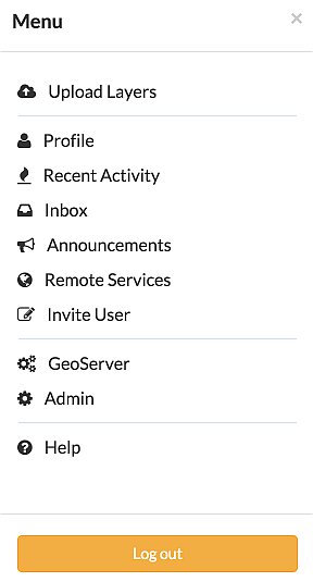
Now you’ve created a superuser you should become familiar with the Django Admin Interface. As a superuser you are having access to this interface, where you can manage users, Datasets, permission and more. To learn more detailed about this interface check this LINK. For now it will be enough to just follow the steps. To attend the Django Admin Interface, go to your geonode website and sign in with your_superuser. Once you’ve logged in, the name of your user will appear on the top right. Click on it and the following menu will show up:
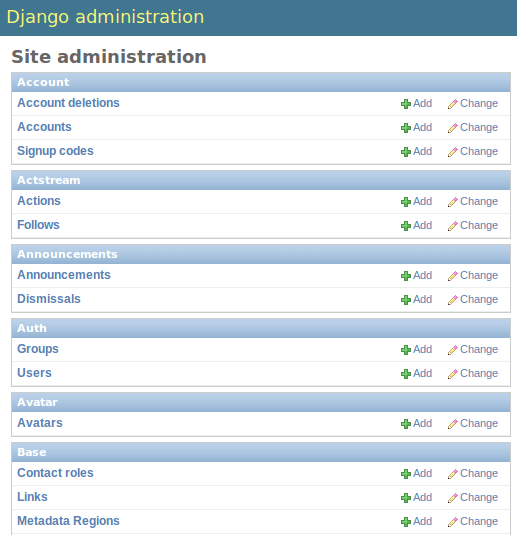
Clicking on Admin causes the interface to show up.
Go to Auth -> Users and you will see all the users that exist at the moment. In your case it will only be your_superuser. Click on it, and you will see a section on Personal Info, one on Permissions and one on Important dates. For the moment, the section on Permissions is the most important.
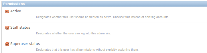
As you can see, there are three boxes that can be checked and unchecked. Because you’ve created a superuser, all three boxes are checked as default. If only the box active would have been checked, the user would not be a superuser and would not be able to access the Django Admin Interface (which is only available for users with the staff status). Therefore keep the following two things in mind:
a superuser is able to access the Django Admin Interface and he has all permissions on the data uploaded to GeoNode.
an ordinary user (created from the GeoNode interface) only has active permissions by default. The user will not have the ability to access the Django Admin Interface and certain permissions have to be added for him.
Until now we’ve only created superusers. So how do you create an ordinary user? You have two options:
Django Admin Interface
First we will create a user via the Django Admin Interface because we’ve still got it open. Therefore go back to Auth -> Users and you should find a button on the right that says Add user.

Click on it and a form to fill out will appear. Name the new user test_user, choose a password and click save at the right bottom of the site.
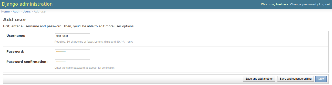
Now you should be directed to the site where you could change the permissions on the user test_user. As default only active is checked. If you want this user also to be able to attend this admin interface you could also check staff status. But for now we leave the settings as they are!
To test whether the new user was successfully created, go back to the GeoNode web page and try to sign in.
GeoNode website
- To create an ordinary user you could also just use the GeoNode website. If you installed GeoNode using a release, you should
see a Register button on the top, beside the Sign in button (you might have to log out before).

Hit the button and again a form will appear for you to fill out. This user will be named geonode_user
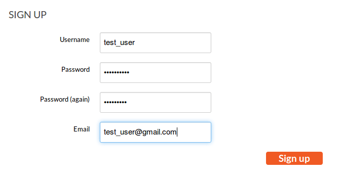
By hitting Sign up the user will be signed up, as default only with the status active.
Batch Sync Permissions
GeoNode provides a very useful management command set_layers_permisions allowing an administrator to easily add / remove permissions to groups and users on one or more Datasets.
The set_layers_permisions command arguments are:
permissions to set/unset –> read, download, edit, manage
READ_PERMISSIONS = [
    'view_resourcebase'
]
DOWNLOAD_PERMISSIONS = [
    'view_resourcebase',
    'download_resourcebase'
]
EDIT_PERMISSIONS = [
    'view_resourcebase',
    'change_dataset_style',
    'download_resourcebase',
    'change_resourcebase_metadata',
    'change_dataset_data',
    'change_resourcebase'
]
MANAGE_PERMISSIONS = [
    'delete_resourcebase',
    'change_resourcebase',
    'view_resourcebase',
    'change_resourcebase_permissions',
    'change_dataset_style',
    'change_resourcebase_metadata',
    'publish_resourcebase',
    'change_dataset_data',
    'download_resourcebase'
]
NB: the above permissions list may change with the ADVANCED_WORKFLOW enabled. For additional info: https://docs.geonode.org/en/master/admin/admin_panel/index.html#how-to-enable-the-advanced-workflow
resources (Datasets) which permissions will be assigned on –> type the Dataset id, multiple choices can be typed with comma separator, if no ids are provided all the Datasets will be considered
users who permissions will be assigned to, multiple choices can be typed with a comma separator
groups who permissions will be assigned to, multiple choices can be typed with a comma separator
delete flag (optional) which means the permissions will be unset
Usage examples:
Assign edit permissions on the Datasets with id 1 and 2 to the users username1 and username2 and to the group group_name1.
python manage.py set_layers-permissions -p edit -u username1,username2 -g group_name1 -r 1,2
Assign manage permissions on all the Datasets to the group group_name1.
python manage.py set_layers-permissions -p manage -g group_C
Unset download permissions on the Dataset with id 1 for the user username1.
python manage.py set_layers-permissions -p download -u username1 -r 1 -d
The same functionalities, with some limitations, are available also from the Admin Dashboard >> Users or Admin Dashboard >> Groups >> Group profiles.
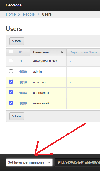
An action named Set layer permissions is available from the list, redirecting the administrator to a form to set / unset read, edit, download permissions on the selected Users/group profile.
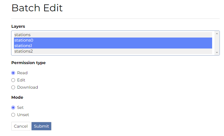
Is enough to select the dataset and press “Submit”. If the async mode is activated, the permission assign is asyncronous
Delete Certain GeoNode Resources
The delete_resources Management Command allows to remove resources meeting a certain condition,
specified in a form of a serialized django Q() expression.
First of all let’s take a look at the --help option of the delete_resources
management command in order to inspect all the command options and features.
Run
DJANGO_SETTINGS_MODULE=geonode.settings python manage.py delete_resources --help
Note
If you enabled local_settings.py the command will change as following:
DJANGO_SETTINGS_MODULE=geonode.local_settings python manage.py delete_resources --help
This will produce output the following output:
usage: manage.py delete_resources [-h] [-c CONFIG_PATH]
                                  [-l LAYER_FILTERS [LAYER_FILTERS ...]]
                                  [-m MAP_FILTERS [MAP_FILTERS ...]]
                                  [-d DOCUMENT_FILTERS [DOCUMENT_FILTERS ...]]
                                  [--version] [-v {0,1,2,3}]
                                  [--settings SETTINGS]
                                  [--pythonpath PYTHONPATH] [--traceback]
                                  [--no-color] [--force-color]

Delete resources meeting a certain condition

optional arguments:
  -h, --help            show this help message and exit
  -c CONFIG_PATH, --config CONFIG_PATH
                        Configuration file path. Default is:
                        delete_resources.json
  -l LAYER_FILTERS [LAYER_FILTERS ...], --layer_filters LAYER_FILTERS [LAYER_FILTERS ...]
  -m MAP_FILTERS [MAP_FILTERS ...], --map_filters MAP_FILTERS [MAP_FILTERS ...]
  -d DOCUMENT_FILTERS [DOCUMENT_FILTERS ...], --document_filters DOCUMENT_FILTERS [DOCUMENT_FILTERS ...]
  --version             show program's version number and exit
  -v {0,1,2,3}, --verbosity {0,1,2,3}
                        Verbosity level; 0=minimal output, 1=normal output,
                        2=verbose output, 3=very verbose output
  --settings SETTINGS   The Python path to a settings module, e.g.
                        "myproject.settings.main". If this isn't provided, the
                        DJANGO_SETTINGS_MODULE environment variable will be
                        used.
  --pythonpath PYTHONPATH
                        A directory to add to the Python path, e.g.
                        "/home/djangoprojects/myproject".
  --traceback           Raise on CommandError exceptions
  --no-color            Don't colorize the command output.
  --force-color         Force colorization of the command output.
There are two ways to declare Q() expressions filtering which resources should be deleted:
With a JSON configuration file: passing
-cargument specifying the path to the JSON configuration file.
Example 1: Relative path to the config file (to
manage.py)DJANGO_SETTINGS_MODULE=geonode.settings python manage.py delete_resources -c geonode/base/management/commands/delete_resources.json
Example 2: Absolute path to the config file
DJANGO_SETTINGS_MODULE=geonode.settings python manage.py delete_resources -c /home/User/Geonode/configs/delete_resources.json
With CLI: passing
-l-d-mlist arguments for each of resources (Datasets, documents, maps)
Example 3: Delete resources without configuration file
DJANGO_SETTINGS_MODULE=geonode.settings python manage.py delete_resources -l 'Q(pk__in: [1, 2]) | Q(title__icontains:"italy")' 'Q(owner__name=admin)' -d '*' -m "Q(pk__in=[1, 2])"
Configuration File
The JSON configuration file should contain a single filters object, which consists of Dataset, map and document lists.
Each list specifies the filter conditions applied to a corresponding queryset, defining which items will be deleted.
The filters are evaluated and directly inserted into Django .filter() method, which means the filters occurring as
separated list items are treated as AND condition. To create OR query | operator should be used. For more info please check Django
[documentation](https://docs.djangoproject.com/en/3.2/topics/db/queries/#complex-lookups-with-q-objects)).
The only exception is passing a list with '*' which will cause deleting all the queryset of the resource.
Example 4: Example content of the configuration file, which will delete Datasets with ID’s 1, 2, and 3, those owned by admin user, along with all defined maps.
{
  "filters": {
  "Dataset": [
      "Q(pk__in=[1, 2, 3]) | Q(title__icontains='italy')",
      "Q(user__name=admin)"
    ],
  "map": ["*"],
  "document": []
  }
}
CLI
The CLI configuration can be specified with -l -d -m list arguments, which in fact are a translation
of the configuration JSON file. -l -d -m arguments are evaluated in the same manner as filters.Dataset,
filters.map and filter.document accordingly from the Example 4.
The following example’s result will be equivalent to Example 4:
Example 5: Example CLI configuration, which will delete Datasets with ID’s 1, 2, and 3, along with all maps.
DJANGO_SETTINGS_MODULE=geonode.settings python manage.py delete_resources -l 'Q(pk__in: [1, 2, 3]) | Q(title__icontains:"italy")' 'Q(owner__name=admin)' -m '*'
Async execution over http
It is possible to expose and run management commands over http.
To run custom django management commands usually we make make use of the command line:
python manage.py ping_mngmt_commands_http
$> pong
The management_commands_http app allows us to run commands when we have no access to the command line.
It’s possible to run a command using the API or the django admin GUI.
For security reasons, only admin users can access the feature and the desired command needs to be explicitly exposed. By default the following commands are exposed: ping_mngmt_commands_http, updatelayers, sync_geonode_datasets, sync_geonode_maps, importlayers and set_all_datasets_metadata.
To expose more command you can change the environment variable MANAGEMENT_COMMANDS_EXPOSED_OVER_HTTP and the added commands will be exposed in your application.
The list of exposed commands is available by the endpoint list_management_commands and also presented by the form in the admin page create management command job.
Note
To use the commands in an asyncronous approach ASYNC_SIGNALS needs to be set to True and celery should be running.
Manage using django admin interface
Creating a job
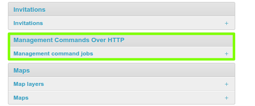
Access the admin panel: http://<your_geonode_host>/admin and go to “Management command jobs”.
Management command admin section
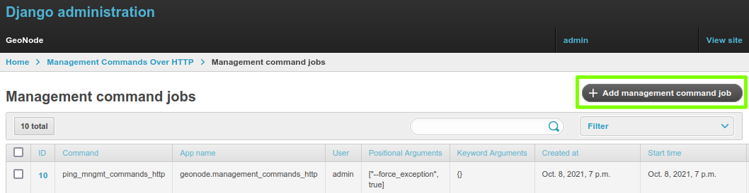
You will arrive at http://<your_geonode_host>/en/admin/management_commands_http/managementcommandjob/,
then click on the buttton + Add management command job (http://<your_geonode_host>/en/admin/management_commands_http/managementcommandjob/add/).
Add management command job
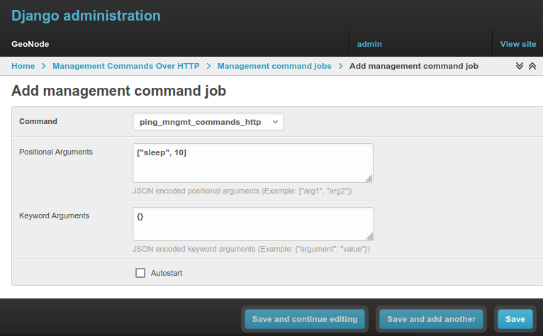
Select the command and fill the form, with the arguments and/or key-arguments if needed.
Save you job and in the list select the start action, alterantively you can mark the autostart option and the command will be automatic started when created.
Creating a management command job form
Starting a job
To start a job:
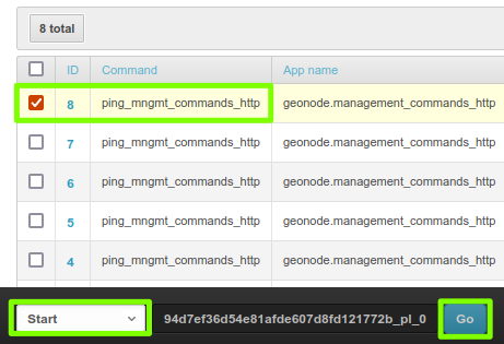
Starting a job
Select the job to be started.
Select the
startaction.Click in
Go.The page will refresh and the job status will have changed. If it takes a long to run, refresh the page to see the updated the status.
A
stopoption is also available.
Note
If it takes too long to load the page, ASYNC_SIGNALS may not be activated.
If its status gets stuck at QUEUED, verify if celery is running and properly configured.
Job status
Clicking at the link in the ID of a job, we can see the details of this job. For the job we just created, we can verify the output message and celery job status.
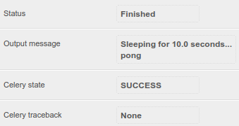
Example job status
When we have an error during execution the traceback message will be available in the Celery traceback.
In the next image a ping_mngmt_commands_http job was created with the arguments ["--force_exception", true].
Checking the text in this field can be useful when troubleshooting errors.
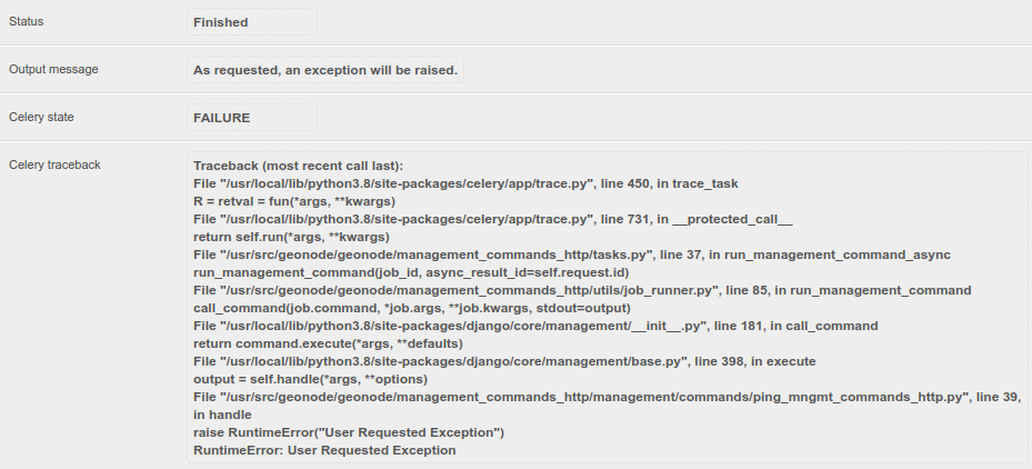
Example job traceback message
Manage using API endpoints
The execution of the management commands can be handled by http requests to an API: http://<your_geonode_host>/api/v2/management/.
All the requests need to be authenticated with administrative permissions (superuser).
You can find here a postman collection with all the exemples listed here and other available endpoints:
geonode_mngmt_commands.postman_collection.json
List exposed commands
Getting a list of the exposed commands:
curl --location --request GET 'http://<your_geonode_host>/api/v2/management/commands/' --header 'Authorization: Basic YWRtaW46YWRtaW4='
Response:
{
    "success": true,
    "error": null,
    "data": [
        "ping_mngmt_commands_http",
        "updatelayers",
        "set_all_datasets_metadata",
        "sync_geonode_maps",
        "importlayers",
        "sync_geonode_datasets"
    ]
}
Note
You should change the header Authorization (Basic YWRtaW46YWRtaW4=) to your Auth token, in this example I am using a token for admin as username and admin as password.
Creating a job
Optionally, before creating the job you can get its help message with the following call:
curl --location --request GET 'http://<your_geonode_host>/api/v2/management/commands/ping_mngmt_commands_http/' --header 'Authorization: Basic YWRtaW46YWRtaW4='
Creating a job for running ping_mngmt_commands_http with 30 seconds of sleep time:
curl --location --request POST 'http://<your_geonode_host>/api/v2/management/commands/ping_mngmt_commands_http/jobs/' \
--header 'Authorization: Basic YWRtaW46YWRtaW4=' \
--header 'Content-Type: application/json' \
--data-raw '{
    "args": ["--sleep", 30],
    "kwargs": {},
    "autostart": false
}'
Response:
{
    "success": true,
    "error": null,
    "data": {
        "id": 8,
        "command": "ping_mngmt_commands_http",
        "app_name": "geonode.management_commands_http",
        "user": 1000,
        "status": "CREATED",
        "created_at": "2021-10-08T18:17:25.045752Z",
        "start_time": null,
        "end_time": null,
        "args": [
            "--sleep",
            30
        ],
        "kwargs": {},
        "celery_result_id": null,
        "output_message": null
    }
}
Note
Alterantively you can omit the jobs part of the url to create a job. (Using http://<your_geonode_host>/api/v2/management/commands/ping_mngmt_commands_http/ as url)
Start/Stop actions
To start the created job:
curl --location --request PATCH 'http://<your_geonode_host>/api/v2/management/jobs/8/start/' --header 'Authorization: Basic YWRtaW46YWRtaW4='
Response:
{
    "success": true,
    "error": null,
    "data": {
        "id": 8,
        "command": "ping_mngmt_commands_http",
        "app_name": "geonode.management_commands_http",
        "user": 1000,
        "status": "QUEUED",
        "created_at": "2021-10-08T18:17:25.045752Z",
        "start_time": null,
        "end_time": null,
        "args": [
            "--sleep",
            30
        ],
        "kwargs": {},
        "celery_result_id": null,
        "output_message": null
    }
}
Note
During execution the job can be interrupted using the following call:
curl --location --request PATCH 'http://<your_geonode_host>/api/v2/management/jobs/8/stop/' --header 'Authorization: Basic YWRtaW46YWRtaW4='
Note that the status changed from CREATED to QUEUED, during execution it will be STARTED and at the end FINISHED.
Jobs list and status
You can verify your job status and details with the following call:
curl --location --request GET 'http://<your_geonode_host>/api/v2/management/jobs/8/status/' --header 'Authorization: Basic YWRtaW46YWRtaW4='
Response:
{
    "id": 8,
    "command": "ping_mngmt_commands_http",
    "app_name": "geonode.management_commands_http",
    "user": 1000,
    "status": "FINISHED",
    "created_at": "2021-10-08T18:17:25.045752Z",
    "start_time": "2021-10-08T18:20:02.761475Z",
    "end_time": "2021-10-08T18:20:32.802007Z",
    "args": [
        "--sleep",
        30
    ],
    "kwargs": {},
    "celery_result_id": "fe7359a6-5f8c-47bf-859a-84351b5ed80c",
    "output_message": "Sleeping for 30.0 seconds...\npong\n",
    "celery_task_meta": {
        "date_done": "2021-10-08T18:20:32.810649Z",
        "status": "SUCCESS",
        "traceback": null,
        "worker": "worker1@4f641ffa9c0b"
    }
}
When runing multiple jobs and to audit already ran jobs. A list of jobs can be retrieved using the following call:
curl --location --request GET 'http://<your_geonode_host>/api/v2/management/jobs/' --header 'Authorization: Basic YWRtaW46YWRtaW4='
Response:
{
    "links": {
        "next": null,
        "previous": null
    },
    "total": 1,
    "page": 1,
    "page_size": 10,
    "data": [
        {
            "id": 1,
            "command": "ping_mngmt_commands_http",
            "app_name": "geonode.management_commands_http",
            "user": 1000,
            "status": "FINISHED",
            "created_at": "2021-10-08T18:17:25.045752Z"
        }
    ]
}
Note
This list can be filtered by the fields “celery_result_id”, “command”, “app_name”, “status”, “user” and “user__username”.